


The MIPSGAL survey consists of 24 and 70 micron obseravtions, obtained through the MIPS instrument on the Spitzer Space Telescope. Both bands suffer from numerous artifacts that are rectified through multiple steps of processing.
24 Micron Image Processing
The MIPSGAL team starts with the raw data and calibration files provided by the Spitzer Science Center (SSC). We run our own version of the basic calibrated data (BCD) pipeline which contains two improvements over the current SSC pipleine (version S16.1). The first improvement is a mode robust identification of very saturated (but not hard saturated) pixels. The second is an improved droop correction for bright pixels. We perform the droop correction separately for the first difference data using the slope values for data which is below the threshold. The MIPSGAL pipeline is written in IDL, operates on multiple AOR directories at a time and requires both the raw and cal subdirectories for a given AOR. The code is available on request.
The two main types of artifacts that are generated by scanning across bright point sources and compact extended emission are latency and global effects. Latency effects are a result of short timescale elevations and long timescale depressions in pixels that have experienced high flux levels. The global effects are where entire columns or rows of pixels have level offsets due to the presence of a bright source on or adjacent to the array. The MIPSGAL team characterizes the artifacts and determine a correction. In some cases, the the artifacts are simply masked from the images.
Jailbars
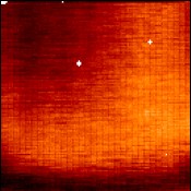
The Artifact: The 128x128 Si:As array is read out in four
groups of alternating columns. A very bright localized source will
typically depress the output of each readout differently by an amount dependent
in some way on the brightest pixel in the readout, creating a vertical-bar pattern in the image.
The depression level can also differ before and after the triggering bright pixel,
so the pattern can be different above and below the source.
The Fix: The array is divided into horizontal
sections, with the presumptive triggering sources as the boundaries.
Within each section, the correction is initially determined row by row:
For each row, any true background trending is removed by smoothing the row
over a 4-pixel window (averaging the readouts) and subtracting from the
original row. The median of the 32 pixels in the row for each readout is
calculated. The peak median is considered “truth” (as the
artifact is always a depression), and the offset adjustments for the
remaining three readouts needed to match the truth are the corrections for
that readout for that row. A linear trending is fit to all the
row-corrections for each readout in that section; the fit gives the
readout corrections for that section.
sample jailbar
Washboard
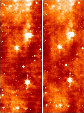
The Artifact: The 128x128 array exhibits a
depression in levels across an irregular band typically about 10-20 pixels
in width at the bottom of the array. The depression is about 1 MJy/sr.
With the ~1/6 array vertical shift per BCD image in each scan leg, this
produces cross-scan banding in the composite images at about 1 arcminute
spatial period. The averaging reduces the amplitude of the effect but it
is still very apparent at low background levels.
The Fix: The effect is assumed to be an
offset, and is assumed to be fixed for a given AOR, but may vary from AOR
to AOR. If the artifact was a gain effect, the depression level would vary
significantly over the large dynamic range in the background for a given
MIPSGAL AOR. For each AOR, a “minimum array image” is created that
represents the typical lowest value each pixel attains in the AOR. For
each pixel, the ensemble of ~1000 values throughout the AOR are sorted,
the lowest seven are discarded, and the next 25 are averaged together. The
result should show systematic deviations from uniformity but be generally
free of any true background structure.The zero point is selected as the median level, and is subtracted from
the “minimum image.” The image is then inverted and applied as
an additive correction throughout the AOR.
example washboard
washboard correction
Dark Latents
The Artifact: When a pixel on the array is
illuminated with a very high brightness level (>20,000 MJy/sr or so), the
response of that pixel is depressed modestly (1-2 MJy/sr), and the effect
can persist for hours. For point sources, the threshold is about 25 Jy,
which produces a dark latent artifact a couple of pixels wide, and at
several hundred Janskys the artifacts can be 9 or 10 pixels wide. The net
effect is to produce long sequences of faint dark blobs in composite
images.
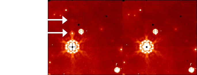
The Fix: The dark latent effect is very
long-lasting, so in a given AOR we can see either pre-existing artifacts
which are seen throughout the AOR, or we can see newly occurring dark
latents, due to crossing a bright source during the AOR, which commence at
some point and persist to the end of the AOR.
The pre-existing dark latents almost always appear in the “minimum image” calculated for the “washboard” artifact correction, and are corrected for without further effort. The “minimum image” may also contain, however, newly-occurring dark latents, depending on when and where in the AOR the triggering bright source is crossed. In this case, we need to edit the “washboard” correction image for the BCDs that precede the triggering event. For this purpose, we use the MSX point source catalog and Band E images to estimate times and positions of the point and extended sources that trigger the new dark latents. When these sources fall on a BCD, the “washboard” correction image is edited for the preceding BCDs by replacing the affected pixels with those from a filtered correction image that has had small-scale structure removed.
This leaves the newly-occurring dark latents that don’t
appear in the washboard correction image. To identify these, averages of
groups of BCDs in an AOR are made (to increase “signal to
noise” of the latent images), with all other corrections applied.
The averages are inspected visually, and the remaining dark latents are
identified. The triggering source position and size of the latents are
determined from the original BCDs. For each, a “minimum image”
as for the washboard correction is made but only using the downstream
BCDs. The dark latent image is clipped out of the minimum image, inverted
and applied as a correction to the downstream BCDs.
sample dark latent correction
Array-Edge Sources
The Artifact: When a bright point source falls very
near or even slightly off the sides of the array, the rows of the array
containing or are adjacent to the brightest part of the source profile
have elevated values. The elevation extends from the edge of the array to
about the middle, but for very bright sources can extend across the array.
The net result is to produce one-sided “diffraction
spike”-like artifacts in the composite images.
The Fix: The point sources that suffer this
artifact are identifiable from the initial composite plates (with other
corrections applied). A catalog is made from these sources.
For each BCD, these sources are mapped into the array coordinates. When one of the sources falls near the edge, the rows containing, or are level with, the brightest parts of the source are simply masked out. Currently the entire row is masked, but it should be possible to identify a flux threshold below which it will be sufficient to mask only half the row nearest the source.
Note that if a source falls near the edge, the half-array spacing of the coverage assures that the source will fall near the middle in some other scan, so there should be no gaps in the final composite images. sample masking of stray light
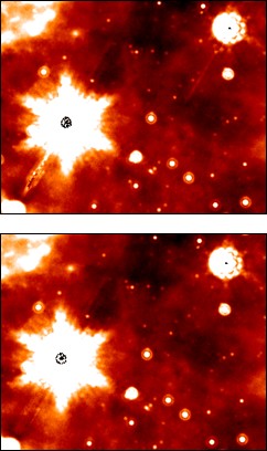
Overlap Corrections
Overlap Corrections
The Artifact: There do not seem to be significant
level differences from AOR to AOR due to, e.g., zodiacal epoch variations.
However, we do see scan leg to scan leg differences particularly at the
ends of the legs, both within AORs and across AORs. Also, we occasionally
see overall elevated levels in BCDs containing bright point sources, and
also within-BCD level mismatches due to severe jailbar effects.
The Fix: The approach is to match levels in the
BCD-to-BCD overlaps. This is done by allowing, as an optimized parameter,
a scalar offset for each BCD. These are optimized by minimizing the sum of
the overlap differences of each BCD with its neighbors. For N BCDs, this
results in N equations linear in the offsets. We can solve for the offsets
for all ~190,000 BCDs in each quadrant simultaneously, in a reasonable
time frame, using sparse matrix operations.
For the BCDs containing the jailbar-induced level differences, these are split into two parts, above and below the triggering source, and each part is entered into the matching process separately. Overlap correction example
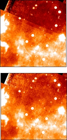
Bright Latents
The Artifact:Pixels in the array retain a “memory” of their values for a given integration in subsequent BCDs, starting at about 1% of the brightness in the following BCD and decreasing quasi-exponentially thereafter. For bright point sources, this can leave a trail of pointlike images as the array scans across the source.
The flux threshold for causing visible latent images is about 100
mJy. Very bright (>100 Jy) sources can leave visible latents for up to
12 subsequent BCDs.
The Fix:The approach is to model the latent
response and subtract the estimated latent levels from the subsequent
images. At lower latent-triggering brightness levels (up to ~2000 MJy/sr),
the latent trigger-response relation can be measured directly. At higher
levels, the trigger pixel is saturated but can be estimated from the known
PRF. The latent brightness function for the first two integration
intervals following a triggering event are thus measured empirically, and
have been modeled as an exponential + linear function of the triggering
brightness, with a ceiling also imposed (see figure at right). The
remaining latent intervals are estimated by scaling the second interval
function.
To apply a correction, the BCDs for a given AOR are stepped through. For a given BCD, the non-saturated pixel brightnesses are recorded and a latent image is calculated from the model (all pixels get some correction). The latent image is then subtracted from the subsequent BCD.
Saturated point sources require special handling. A catalog of
these sources (greater than ~2 Jy) is first prepared, with estimates of
flux and position from a PRF fit using the wings of the response function.
For each BCD, the saturated sources are projected into the array using the
known PRF, and the true incident brightnesses of the saturated pixels are
estimated from the PRF, and are used as the latent triggering values.
sample bright latents correction
+ 70 Micron Image Processing
Will be filled in soon.